Introduction
Continuing the discussion of spectral biclustering methods, this post covers the Spectral Biclustering algorithm (Kluger, et. al., 2003) [1]. This method was originally formulated for clustering tumor profiles collected via RNA microarrays. This section introduces the checkerboard bicluster structure that the algorithm fits. The next section describes the algorithm in detail. Finally, in the last section we will see how it can be used for clustering real microarray data.
The data collected from a gene expression microarray experiment may be arranged in a matrix $A$, where the rows represent genes and the columns represent individual microarrays. Entry $A_{ij}$ measures the amount of RNA produced by gene $i$ that was measured by microarray $j$. If each microarray was used to measure tumor tissue, then each column of $A$ represents the gene expression profile of that tumor.
For each kind of tumor, we expect subsets of genes to behave differently. For instance, in Liposarcoma a certain subset of genes may be highly active, while in Chondrosarcoma that same subset of genes may show almost no activity. Assuming these patterns of differing expression levels are consistent, then the data would exhibit a checkerboard pattern. Each block represents a subset of genes that is similarly expressed in a subset of tumors.
Let us see an artificial example, using the following matrix.
Rearranging the rows and columns of the original matrix reveals the checkerboard pattern.
The Spectral Biclustering algorithm was created to find these checkerboard patterns, if they exist. Let us see how it works.
The algorithm
To motivate the algorithm, let us start with a perfect checkerboard matrix $A$. Let us also assume we have row and column classification vectors $x$ and $y$, with piecewise-constant values corresponding to the row and column partitions of the matrix. Then applying $A$ to $c$ yields a new row classification vector $r’$ with the same block pattern as the original, and vice versa:
$$A c = r’ \\
A^{\top} r = c’$$
Substitution gives:
$$A A^{\top} r = r’ \\
A^{\top} A c = c’$$
where $r$, $r’$, $c$, and $c’$ are not necessary the same as in the previous equations. These equations look like the coupled eigenvalue problem:
$$A A^{\top} r = \lambda^2 r \\
A^{\top} A c = \lambda^2 c$$
where eigenvectors $r$ and $c$ have the same eigenvalue $\lambda^2$. This problem can be solved via the singular value decomposition. So if the matrix has a checkerboard structure, a pair of singular vectors will give us the appropriate row and column classification vectors. This is the heart of the algorithm.
Before applying the SVD, however, it is useful to normalize the matrix to make the checkerboard pattern more obvious. For instance, if each row has been multiplied by a different scaling factor, applying the matrix to the column classification vector gives a noisy row classification vector. If we first scale each row of the matrix so that they have the same mean, the resulting row classification vector will be closer to a piecewise-constant vector.
It turns out that we can perform this scaling using the diagonal matrix $R^{-\frac{1}{2}}$ that we first saw in the `last post last post. Similarly, we can scale the columns using $C^{-\frac{1}{2}}$. Therefore, we can enhance the checkerboard pattern by normalizing the matrix to $A_n = R^{-\frac{1}{2}} A C^{-\frac{1}{2}}$, exactly in Dhillon’s Spectral Co-Clustering algorithm. The rows of matrix $A_n$ all share the same mean, and its columns share a different mean.
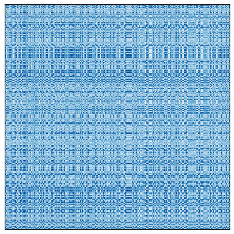
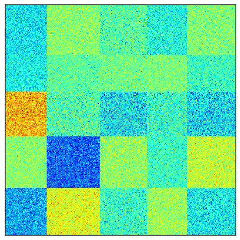
To demonstrate how normalization can be useful, here is a visualization of perfect checkerboard a matrix in which each row and column has been multiplied by some random scaling factor.
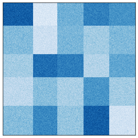
After normalization, the checkerboards are more uniform:
Kluger, et. al., introduced another normalization method, which they called bistochastization. This method makes all rows and all columns have the same mean value. Matrices with this property are called bistochastic. In this method, the matrix is repeatedly normalized until convergence. The first step is the same:
$$A_1 = R_0^{-\frac{1}{2}} A C_0^{-\frac{1}{2}}$$
Each subsequent step repeats the normalization of the matrix obtained in the previous step:
$$A_{t+1} = R_t^{-\frac{1}{2}} A_t C_t^{-\frac{1}{2}}$$
Again, let us visualize the result of normalizing the original matrix.
Bistochastization makes the pattern even more obvious.
Finally, Kluger, et. al., also introduced a third method, log normalization. First, the log of the data matrix is computed, $L = \log A$, then the final matrix is computed according to the formula:
$$K_{ij} = L_{ij} - \overline{L_{i \cdot}} - \overline{L_{\cdot j}} + \overline{L_{\cdot \cdot}}$$
where $\overline{L_{i \cdot}}$ is the column mean, $\overline{L_{\cdot j}}$ is the row mean, and $\overline{L_{\cdot \cdot}}$ is the overall mean of $L$. This transformation removes the systematic variability among rows and columns. The remaining value $K_{ij}$ captures the interaction between row $i$ and column $j$ that cannot be explained by systematic variability among rows, among columns, or within the entire matrix.
An interesting consequence of this method is that adding a positive constant to $K$ makes the it bistochastic.
To visualize the result, we first transform the matrix by taking $\exp(A)$.
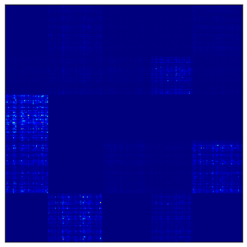
Then the log normalization reveals the checkerboard pattern.
After the matrix has been normalized according to one of these methods, its first $p$ singular vectors are computed, as we have seen earlier. Now the problem is to somehow convert these singular vectors into partitioning vectors.
If log normalization was used, all the singular vectors are meaningful, because the contribution of the overall matrix has already been discarded. If independent normalization or bistochastization were used, however, the first singular vectors $u_1$ and $v_1$ are discarded. From now on, the “first” singular vectors refers to $U = [u_2 \dots u_{p+1}]$ and $V = [v_2 \dots v_{p+1}]$ except in the case of log normalization.
There are two methods described in the paper for converting these singular vectors into row and column partitions. Both rely on determining the vectors that can be best approximated by a piecewise-constant vector. In my implementation, the approximations for each vector are found using one-dimensional k-means, and the best are found using the Euclidean distance between each vector and its approximation.
In the first method, the best left singular vector $u_b$ determines the row partitioning and the best right singular vector $v_b$ determines the column partitioning. The assignments of rows and columns to biclusters is determined by the k-means clustering of $u_b$ and $v_b$.
The second method is the one I chose to implement. In this method, the data is projected to the best subset of singular vectors. For instance, if $p$ singular vectors were calculated, the $q$ best are found as described, where $q<p$. Let $U_b$ be the matrix with columns the $q$ best left singular vectors, and similarly $V_b$ for the right. To partition the rows, the rows of $A$ are projected to a $q$ dimensional space: $A V_{b}$. Treating the $m$ rows of this $m \times q$ matrix as samples and clustering using k-means yields the row labels. Similarly, projecting the columns to $A^{\top} U_{b}$ and clustering this $n \times q$ matrix yields the column labels.
Here, then, is the complete algorithm. First, normalize according to one of the three methods:
- Independent row and column normalization: $A_n = R^{-\frac{1}{2}} A C^{-\frac{1}{2}}$
- Bistochastization: repeated row and column normalization until convergence.
- Log normalization: $K_{ij} = L_{ij} - \overline{L_{i \cdot}} - \overline{L_{\cdot j}} + \overline{L_{\cdot \cdot}}$
Then compute the first few singular vectors, $U$ and $V$. Determine the best subset, $U_b$ and $V_b$. Project the rows to $A V_b$ and cluster using k-means to obtain row partitions. Project the columns to $A^{T} U_b$ and cluster using k-means to obtain the column partitions.
Example: clustering microarray data
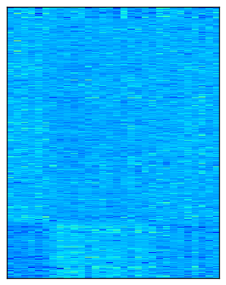
Now we will demonstrate the algorithm on a real microarray dataset from the Gene Expression Omnibus (GEO). Here we download and cluster GDS4407, which contains gene expression profiles of mononuclear blood cells of thirty patients: eleven have acute myeloid leukemia (AML), another nine have AML with multilineage dysplasia, and ten are the control group. Since there are three types of samples, we will try to cluster the data into a $3 \times 3$ checkerboard.
import urllib
import gzip
import numpy as np
from Bio import Geo
from sklearn.cluster.bicluster import SpectralBiclustering

# download and parse text file
name = "GDS4407"
filename = "{}.soft.gz".format(name)
url = ("ftp://ftp.ncbi.nlm.nih.gov/"
       "geo/datasets/GDS4nnn/{}/soft/{}".format(name, filename))

urllib.urlretrieve(url, filename)
handle = gzip.open(filename)
records = list(Geo.parse(handle))
handle.close()
data = np.array(list(map(float, row[2:])
                     for row in records[-1].table_rows[1:]))

# do clustering
model = SpectralBiclustering(3, method="bistochastic", random_state=0)
model.fit(data)
This code requires BioPython for parsing the text file downloaded from the GEO. Note that the method used here for downloading the data and converting it to a NumPy array is ad-hoc and probably fragile. The fitting step took 6.91 seconds on a laptop with a Core i5-2520M processor.
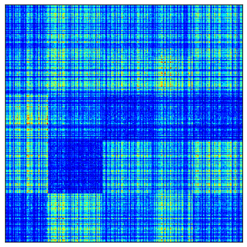
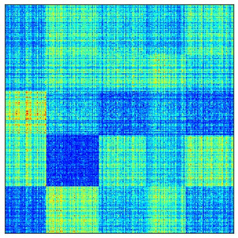
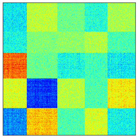
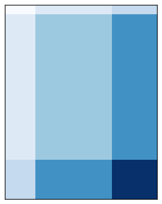
Here is a visualization of the checkerboard pattern found by the model, followed by the corresponding rearrangement of the data, normalized by bistochastization:
As I mentioned in the last post, this implementation will eventually be available in scikit-learn. In the meantime, it is available in my personal branch.
Conclusion
We have now covered both spectral biclustering methods. As you have seen, there are some similarities between them. Both involve normalizing the data, finding the first few singular vectors, and using k-means to partition the rows and columns.
The methods differ in their bicluster structure. In fact, the checkerboard structure may have a different number of row clusters than column clusters, whereas the Spectral Co-Clustering algorithm requires that they have the same number. The methods also differ in how many singular vectors they use and how they project and cluster the rows and columns. Spectral Co-Clustering simultaneously projects and clustered rows and columns, whereas Spectral Biclustering does each separately.
Like the other algorithms we have seen, the Spectral Biclustering algorithm was developed to address a specific problem – in this case, analyzing microarray data – but it can be applied to any data matrix.
In the next post we will return to microarrays in order to cover the first biclustering algorithm developed specifically for microarray data: Cheng and Church.
References
[1] Kluger, Y., Basri, R., Chang, J. T., & Gerstein, M. (2003). Spectral biclustering of microarray data: coclustering genes and conditions. Genome research, 13(4), 703-716.